Raster Modelling Part II

Python Script

The second part of this exercise included writing a python script that could generate a new raster overlay based on the same criteria, but with one weighted more heavily than the others. I chose to weight distance from streams higher. It is shown below.

Raster Modeling

Goals and Objectives:

The goal of this exercise was to use a number of geoprocessing tools to build a suitability model and a environmental/social risk model for sand mining in a selected area of interest in Trempealeau county, Wisconsin. The three main tasks were to: 1) Build a sand mining suitability model 2) Build a sand mining risk model 3) Overlay results to determine best locations for potential mining operations

Data Sets/ Sources:

The data used included data from the Trempealeau county public geodatabase, USGS DEM data, NLCD land use data, and water table data from the Wisconsin Geological and Natural History Survey.

Methods:

Before using geoprocessing tools, it is important to make sure that the workspace is set up accordingly. I used a boundary file delimiting my area of interest to limit all raster functions to that boundary, and reduced my processing extent to it as well. 

Suitability Model

The first objective was to find suitable land based on geological criterion. Based on previous knowledge and research, I knew which geologic formations were most desirable for sand mining. I converted a Trempealeau county geology feature class to a raster, then performed a reclass on it, ranking each geologic formation based on their desirability. The process is shown in the below model.

The second objective was to find suitable land based on land use. I ranked each land use type based on what I believed was most suitable using the reclassify tool.

For Barren Land/Herbaceuous/Hay/Pasture/Cultivated Crops I assigned a 3.

For Shrub/Scrub I assigned a 2.

For Deciduous Forest/Evergreen Forest/Mixed Forest I assigned a 1.

For Open Water/Developed, Open Space/Developed, Low Intensity/Developed, Medium Intensity/Developed, High Intensity/Woody Wetlands I assigned 0 to exclude these unusable land types. 

The third objective was to find suitable land based on the proximity to railroad terminals. I performed a Euclidean distance tool, and assigned values of 1, 2, and 3 using reclassify.

The fourth objective was to find suitable land based on slope. I ran the slope calculator tool on the Trempealeau county DEM file, giving me a % rise, then used a block statistics tool to remove the "salt and pepper" effect and average out the slope values. Then, I ranked and reclassed it.

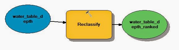
The fifth objective was to rank more highly areas where the water table is closer to the surface. This involved downloading coverage files from WI Geological Survey website and imporing them into my geodatabase before generating a raster from the contour lines using the topo to raster tool. I ranked and reclassed the results again here.

The sixth objective was to combine all of these criteria rasters into one index model that adds up all of the ranks I had assigned in each of them. This involved using raster calculator to add up each raster. The resulting suitability map is shown below in the results section.

Objective seven included removing the exclude land uses, but I had already done this as a part of objective two.

Impact Model

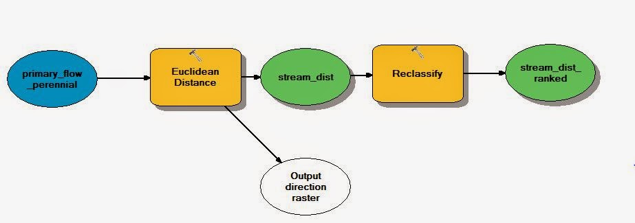
Objective eight included using a DNR hydro feature class to determine environmental impact of potential sand mining operations. I only included primary flow perennial streams. I then used the euclidean distance tool to calculate and reclassify the distances- with 3 having the biggest environmental impact. 

For the ninth objective, I projected a prime farmland feature class, and converted it to raster. Next I used reclass to rank based on land that was prime farmland, or at least valuable farmland. 

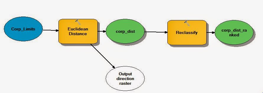
Objective ten involved determining impact based on distance to residential or populated areas. For this, I used a feature class containing corporate boundaries of municipalities. Next, I performed euclidean distance on it, assigning the minimum break a value of 640m, as that is the distance at which a mine cannot be built. These distance classifications were meant to represent a dust shed for potential mines.

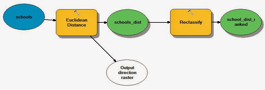
Objective eleven was to determine potential impact on schools. This meant going into the parcels feature class, and querying all parcels with an owner that contained the word 'school' After this, I created a new feature class based on my selection, used the euclidean distance tool, and reclassified the results into rankings. 

For objective twelve, I was able to choose a factor of my choice, and use geoprocessing analysis to determine impact on it. I chose wildlife areas, and again used the euclidean distance tool and reclassify tool to determine impact rankings based on distance.

Objective thirteen was to calculate risk: this is basically the same step that I performed on the suitability rasters, but this time I am using raster calculator to add up the values in my impact rasters to determine the impact. This map can be viewed below in the results section. 

Objective fourteen was to determine potential visibility of mines from somewhere that could be considered a prime recreational area. For this area, I chose Perrot State Park Campground. I created a layer that just contained this as a point feature, and used the viewshed tool (which uses elevation data) to determine all view-able areas. This map is available in the results section below. 

Objective fifteen, the final objective was to overlay suitability results and the environmental impact results to determine the best and worst locations for sand mining. This involved subtracting my environmental/social impact raster model from the suitability raster model, and using the stretched color ramp to symbolize it. This map is also available in the results section. 

Results:

Viewshed Analysis from Perrot SP Campground in Southern
Trempealeau County, Wisconsin

Discussion:

The results of these exercises were interesting- it is important to keep a number of factors in mind modeling suitability or environmental/human impact of mining. The suitability model ended up showing a large portion of the western section as a suitable environment based on these factors. The impact model shows a similar area, but excludes the municipal areas nearby. The overlay shows that central Trempealeau county could be a good place for sand mines. It is important to note that this analysis is based on inferences that might not represent real world data- rather were generated during analysis. 

Conclusion:

This exercise was valuable because it taught me a lot about raster analysis, and the different ways that it can be used on different variables and factors. The geoprocessing tools allow the analyst to perform simple tasks, and use simple mathematics to make valuable conclusions about raster data. 

Network Analysis: Cost of Sand Mining on Local Roads

Goals and Objectives

The goal of this lab was to become acquainted with the Network Analysis tool, and use it to perform analysis of the impact that sand mining has on the transportation system here in Wisconsin. The general workflow I followed is as follows.

1. Determine which rail terminal each mine will travel to in order to get the sand to a rail car.
2. Determine the most efficient route from the mine to the terminal.
3. Calculate the length of the route by county.
4. Estimate the costs each county will incur for road maintenance due to heavy sand truck traffic.

General Methods

The first step was to use a Python script to select all of the mines that were active, did not have a rail loading station included, and was not within 1.5km of any railroad. This script can be seen in my posting from November 11th. Using this new dataset of mine locations, I then had to add a streets network dataset, and all of the feature classes participating in it. I then added a rail terminals feature class to the map, and remove features that had an air terminal facility by selecting the desired features, and creating a layer from the selection. Then, I used the Network Analyst: closest facility tool to determine routes that trucks shipping sand would take to get to the nearest rail terminal. We then used model builder to visualize our workflow, and make it a reusable process. I essentially went through the same process I just explained, and exported the resulting feature class to a geodatabase. The model is shown below. The next step was to calculate the total road length covered per county. I did this by intersecting the trucking routes with the county boundaries, and summarizing (giving me the total length) based on the county field. From there, I created a new field called COST, and calculated its values based on the assumptions that each sand mine takes 50 truck trips per year to the rail terminal, and costs 2.2 cents per mile of wear and tear on the roads. The equation is as follows: [SUM_Shape_length] * 50 / 1609.344 * .022. Finally, I mapped my results. They are shown below.

Results

This image shows the process I went through in using network analysis to calculate routes
likely taken by trucks shipping frack sand.

This image shows the process taken to calculate the costs incurred by sand-moving trucks

This image shows my final results. Counties with higher impact by sand mining transportation
operations are shown in darker colors.

This image shows the table with total length of roads (in meters) affected by sand mine
transportation, and the cost associated with these values.

Discussion

After analyzing the results of this excersise, I am quite surprised at how low the annual costs on the roads are. It is important to note that the assumptions talked about in previous sections (being that each mine takes 50 truck trips per year, and that the cost per truck mile is 2.2cents) is hypothetical. More testing and analysis would be needed in order to make an accurate claim about the monetary implications that frac sand mining has on the transportation system here in WI.

Another important issue with the assumptions is that instead of calculating for 50 trips, I should have calculated for 100, accounting for the trip back from the rail terminal.

Conclusion

 

This lab was a good introduction to using network analysis, and a good way to familiarize myself with some its possible applications. I think that network analysis is one of the most practical tools that I've used so far in GIS, and I'm sure that it is a very popular area because of its use in routing. It will be a good tool to be familiar with in the future.

Python Script 2

For this script, the objective was to write a number of SQL statements to select mines that meet the following criterion:

• Mine must be active
• Mine must not also be a rail loading station
• Mine must not be within 1.5km of any railroad

The script narrowed down the number of mines to 41 that met the criteria. It is shown below.

Sand Mine Suitability Project: Data Normalization, Geocoding, and Error Assessment

Goals and Objectives

The goal of this exercise was to become familiar with the process of geocoding non-normalized data, and combining it with data from sources that have been geocoded differently. We were assigned to geocode addresses of sand mines, merge our results with results from other students, and compare.

General Methods

We were each assigned a number of sand mines from an excel table to geocode. The first issue was that the addresses we were given were not normalized. Some were in WI PLSS format, and others already had street addresses. To facilitate the geocoding process, I used a PLSS finder online to find a street address for each of the mines that I was assigned. (See below for pre-normalization, and post-normalization tables). Once I had all of my street addresses, I began geocoding, using ArcMap's geocoding tools. While the tool matched some of my addresses automatically, there were a number of them that I used the "Pick address from map" tool to locate. This involved zooming to their location using PLSS quarter quarter section data. Since this data was located on our University's database server, I had to connect in order to use it. After I was connected, I used the DNR's roads dataset, and PLSS data to locate my mines, and match them manually. Once they were all properly geocoded, I exported my results as a shapefile, and put it in a folder that included all of the students' geocoded mine shapefiles, some of which contained the same as mines that I had been assigned. The next step was to merge all of these shapefiles. However, some of the students' files were corrupted, or had been compiled differently, so merging the files was a challenge. I had to merge a few files at a time and repeat until I had a usable dataset. Next, I used the Project tool to project my data to a Wisconsin state system projection. I then queried for all geocoded mines that matched my own, and I used a point distance tool to generate a table of the distances between my points, and other students' points. The problem here was that this generated the distances between each of my points and each of theirs, while I was really only interested in the nearest points from other students to each of mine. I summarized my point distance table on my mine-id field, and included minimum distance to generate a table of my mines and how far the nearest mine mapped by other students was.

Results

This image shows some of my mine addresses. Note the ADDRESS_NORMALIZED
field that I added alongside the Address field after the normalization process

This image shows a table of the minimum distance (in ft) that my mines (INPUT_FID) were
from mines geocoded by other students. 

Discussion

As in any geospatial analysis, there were a number of sources of error in this project. Of course, there was inherent error in the map projection and scale etc, but more important was the operational error associated with data compilation and geocoding. We each had to geocode our mine addresses based on PLSS data. Since many of the mines didn't have an associated street address, we had to search for one and assign it one. This leads to various discrepancies between our datasets, resulting in some values in the table above being quite high. In the process of geocoding, many addresses were automatically matched to their normalized street addresses, but many required further analysis. That meant picking a point from the map for which geocode addresses tool would assign an address. This resulted in high operational error, as depending on where I or another student clicked, the address would be assigned differently. The points that are actually correct are likely ones that originally had a street address, and that the geocoding tool automatically assigned a point correctly to that address. These are points that likely have low distance between them in the above table.  

Conclusion

This lab was a good introduction to the process of data normalization and geocoding. In GIS data often comes from different sources, and there are often discrepancies between datasets that must be addressed before analysis. Having to normalize data that might be in a number of formats is a process that I should be familiar with. It is also good to be familiar with the geocoding process, so I am able to generate spatial data from tabular address data. 

Sand Mine Suitability Project: Data Sources

Goals and Objectives

The goal of this assignment was to become familiar with public web GIS data, importing it into Esri ArcGIS, and designing/implementing database to store it in.

General Methods

There were a number of data sets that we downloaded for use in our suitability data. They are listed below with their respective URLs:
US Department of Transportation - http://www.rita.dot.gov/bts/sites/rita.dot.gov.bts/files/publications/national_transportation_atlas_database/index.html
USGS National Map Viewer – http://nationalmap.gov/viewers.html
MRLC – https://www.mrlc.gov USDA Geospatial Data Gateway – http://datagateway.nrcs.usda.gov Trempealeau County Land Records – https://www.tremplocounty.com/landrecords
USDA NRCS Web Soil – http://websoilsurvey.sc.egov.usda.gov/App/HomePage.htm
Our general process included navigating to the data hub, which was often an online interactive map, searching Trempeleau County, and downloading the desired data based on the county's boundaries. With some of the data we downloaded, it was necessary to use a Python script to load our raster files into our geodatabase, clip them to restrict them to just the county boundary, and project them in the desired Trempeleau County projected coordinate system. Since we downloaded the data from the internet, we kept our compressed .zip files in a temporary workspace, and extracted them to a working folder before loading our actual data into the geodatabase. After the project, I deleted the .zip files and working files because they took up extra space, and were no longer necessary. The resulting datasets are shown below.

Data Accuracy

Conclusion

This lab was very important to understand, because GIS is all about interoperability, and it is necessary to understand the processes involved in data downloading, storage, and management. These processes are very common tasks in the workplace, and I am glad to have been introduced to them. 

Python Scripting

Introduction

Python is an open sourced programming language that focuses on code readability, making it a logical, user friendly option for people who are interested in programming. Esri ArcGIS is fully compatible with Python, allowing users to use Python scripting for custom geoprocessing functionality, database management, and many other useful functions. My first real Python script is shown below.

Exercise 5 Script

This script was used to list the rasters images in the specified folder, project them,
clip them to my area of interest, and load them into my geodatabase

Sand Mining in Western Wisconsin Overview

What is frac sand? Where is it in Wisconsin?

Source: Wisconsin DNR

Frac sand is a specific kind of quartz sand that is used for injection in oil and gas wells. It has been mined for over 100 years (3), but due to recent developments in a new oil and gas extraction method called hydraulic fracturing, it is now in much higher demand. It also appears that this boom will continue (2). This particularly affects western Wisconsin and eastern Minnesota because the best frac sand meets certain requirements. The Wisconsin Geological and Natural History Survey notes that it must be "nearly pure quartz, very well rounded, extremely hard, and of uniform size" to be able to be used in gas and oil extraction.
The image to the right shows the locations of the best sand for use in resource extraction. Note that western Wisconsin has extensive frac sand resources.

So what? Isn't it just sand?

The issue isn't losing our sand, it is the environmental and social implications of sand removal. There are many issues surrounding sand mining here in western Wisconsin, including contamination of air and water supplies. The inhalation of silica sand can cause silicosis, which has been known to lead to cancer, and other health problems. While the DNR monitors the emission of silica dust, there are no regulations in place that protect citizens from it. The DNR also recognizes impacts that the mining operations have on water resources, noting that they consume water for their workers, sometimes pump water to reach sand below the water table, and is used for processing the sand once it has been collected (1). Also, non-metallic mining operations can harm surface water resources via runoff carrying sediment, changing water temperatures, or contamination from human impact that is common in resource extraction. It is also worth noting that top soils are in the way of silica sands, so they must be removed as well.

What does this have to do with GIS?

Many sustainability issues can be viewed from the geospatial lense, and frac sand mining is no different! GIS could be used to model a number of different aspects of sand mining. For example, GIS could simply be used to map locations of mines along with nearby human and environmental features, thus mapping the hazard posed to them due to the proximity of the mines. GIS could also be used to model dispersion of contaminants like silica dust, unwanted sediment, or contaminated water.

Sources:

1. http://dnr.wi.gov/topic/Mines/documents/SilicaSandMiningFinal.pdf
2. http://www.minnpost.com/earth-journal/2014/09/frac-sand-mining-boom-accelerating-and-eluding-regulators-analysis-finds
3. http://wcwrpc.org/frac-sand-factsheet.pdf